Originally posted on 2018
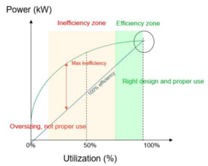
Energy efficiency break even point.
In this post I am going to talk about fine tuning or redesign: energy efficiency break even point . But I’m going to do it in a practical way. So this is the continuation of another post that I wrote, fine tuning or redesign, part 1.
Energy efficiency into practice.
As I mentioned in my first post, I want the blog to be practical and useful. So I will try to explain today’s topic with an example. When do we have to redesign instead of fine tuning? As a summary, in part 1, I concluded that there is a point at which we must move from fine tuning to redesign. Here we will calculate that value.
Suppose we have an installation that pumps water with a centrifugal pump of 40 cubic meters per hour and that consumes 5.5 kilowatts. The price of this pump is 1,700 €. These data are quite approximate to reality.
We measure the efficiency of the system.
We want to know if the system is inefficient. For this we will measure in which area our pump is working. We will measure the flow pumped and the power consumed. We will try to generate the necessary points to represent the theoretical curve of the manufacturer.
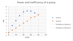

The curve tells us that the consumption when we pump 40 m3/h is 5.5 kW and that when we pump 25 m3/h the consumption is 6.8 kW. We also see, logically, that when we do not pump anything, the consumption is 0 kW. The ideal points, in which there is no inefficiency, are the two extremes. Inefficiency is measured by plotting the ideal consumption, which is a line that joins the two extremes. The distance between the ideal consumption and the real one is inefficiency.
Inefficiency as a function of flow.
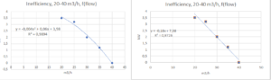
Now we are going to represent the inefficiency versus the pumped flow. It would be the following graph, which corresponds to a quadratic curve.

But to simplify the explanation we are going to focus only on the right part of the bell. We are going to transform it into a polynomial equation and then into a line. With this estimate we increase the error a bit but we gain a lot in simplicity.
Inefficiency is equal to y = -0.18x + 7.38, where x is flow.
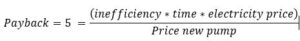
On the other hand we will represent a line that is the price of a new pump versus its flow. We have requested several prices from the manufacturer and we have that a pump of 40 m3/h costs 1,700 € and one of 20 m3/h costs 800 €.
Pump price is y = 45x – 100, where x is the flow.

Company’s payback for approved investments.
In our company the limit to execute an investment is that your payback is equal to 5 years. Therefore, when the annual inefficiency divided by the cost of the pump equals 5 is when we can install a new pump. The formula would be the following.
The pump works 8,700 hours per year and the price of the electricity is 160 €/MW. Clearing the formula we have that the flow for which we have to buy a new pump, redesign, is 22.6 m3/h.
Energy efficiency break even point
That is, if during the normal operation of the system the measured that flow is equal to or less than 22.6 m3/h, then it is more interesting to change the pump than to adjust the system to reduce inefficiencies. The new pump will consume less and will be at the maximum point of consumption and minimum of inefficiency.

Below in the link you will find the excel file with the measurements and graphs:
Fine tune or redesign